Lagrange Error Bound

It's also called the Lagrange Error Theorem, or Taylor's Remainder Theorem.

To approximate a function more precisely, we'd like to express the function as a sum of a Taylor Polynomial & a Remainder.

(▲ For T is the Taylor polynomial with n terms, and R is the Remainder after n terms.)

The tricky part of that expression is to "preset" the accuracy of the Error, aka. the Remainder.

For bounding the Error, out strategy is to apply the Lagrange Error Bound theorem.

Simply saying, the theorem is:

If a function's ALL DERIVATIVES are bounded by a number over the interval (C, x):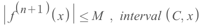
(▲ for C is the centre of approximation)
where the max value of all derivatives of the function is:
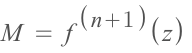
(▲ for z is any value between C and x makes the derivative to the max)
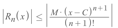
(▲ and note that: the input has to be n+1 )
then the function's Remainder MUST satisfy this theorem:

Example

Solve:

This problem is to approximate a function with Taylor Polynomial.
To do so, we're to set use the Error estimation method, which first to set up the equation: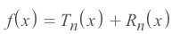
In this case, it is:
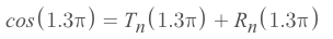
Since it's only asking for the error bound, so we only focus on the Error Rn.
We want to apply the Lagrange Error Bound Theorem, and bound it to 0.001: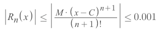
For those unknowns variables in the theorem, we know that:
- The approximation is centred at 1.5π, so C = 1.5π.
- The input of function is 1.3π, so x = 1.3π.
- For The M value, because all the derivatives of the function cos(x), are bounded to 1 even without an interval , so let's say the max value M = 1.
Therefore, the formula of this theorem becomes:
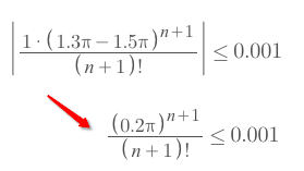
Unfortunately, at this moment we don't have easier method to solve for n except trying some numbers in: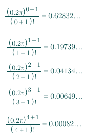
We could see that, with the degree gets larger and larger, the Error becomes smaller and smaller.
Only until n=4, which means the 4th derivative, the Error is less than 0.001.
So the answer is 4th derivative.

Solve:

Same with the problem above, we want to apply the Lagrange Error Bound Theorem, and bound it to 0.001:
For those unknowns variables in the theorem, we know that:
- The approximation is centred at 0 because it's told as a Maclaurin Series , so C = 0.
- The input of function is -0.95, so x = -0.95.
- The interval is (C, x) or (x, C), which is (-0.95, 0) in this case.
For The M value, since all the derivatives of eˣ is just eˣ, and eˣ is unbounded at all, so we're to examine the Max value over the interval (-0.95, 0)
With the help from Desmos Calculator, we know that over the interval (-0.95, 0), the max value of eˣ is e⁰ = 1: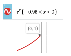
So boundary is M = 1.
Therefore, the formula of this theorem becomes:
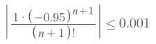
In this case, we need to try some numbers for n to get the desired value: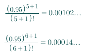
After tried n=5 and n=6, we could see that only until n=6, which means the 6th derivative, the Error is less than 0.001.
So the answer is 6th derivative.

Solve:

Same with the problem above, we want to apply the Lagrange Error Bound Theorem, and bound it to 0.001:
For those unknowns variables in the theorem, we know that:
- The approximation is centred at 2, so C = 2.
- The input of function is 2.5, so x = 2.5.
- The interval then is (2, 2.5).
For the M value, it's not easy to figure out, but we've been told the formula for derivative.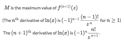
So the expression for M would be:
Let's directly plug in the M expression into the Remainder: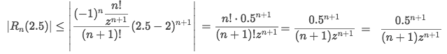
With the help from Desmos grapher we know that when within the interval 2≤ z ≤ 2.5, that z=2 makes the formula to the max: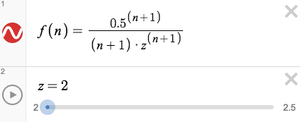
So let's set the inequality:
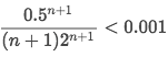
After trying out some number for n, we get that n ≥ 3.

Last updated 5 years ago